Approximating Elliptic Paraboloid by Relu nets
If we regard neural net models as nonparametric approximators of continuous functions, several works are supporting the validity of this method. In particular,
- in reference 1, it has been proved that a one hidden layer neural net with sigmoid activation function can approximate any continuous functions on a unit cube. And later, there are works showing this is also true for Relu activation. The conclusion here is a large flat net is safe to approximate any continuous function.
- in reference 2, oppositely, it shows that with hidden layer widths at most \(w\), and arbitrary depth, Relu nets can approximate any countinous functions. If the net has input dimension \(d_{input}\) and output dimension \(d_{out}\), \(w\) should satisfy \[d_{input}+1 \leq w \leq d_{input}+d_{out}.\] In other words, if all hidden layer widths are bounded by \(d_{input}\), even in the infinite depth limit, Relu nets can only express a very limited class of functions.
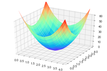
In the following, we will see how Relu nets approximate a Elliptic Paraboloid function with different depth and width.
\[z = 10*(x-2)^2+10*(y-2)^2, x, y \in(0, 4)\times(0, 4)\]
1
2
3
4
5
6
7
import numpy as np
import tensorflow as tf
from tensorflow.python.framework import ops
import matplotlib.pyplot as plt
from matplotlib import cm
from mpl_toolkits.mplot3d import Axes3D
plt.style.use('seaborn-whitegrid')
1
2
3
4
5
6
7
8
9
10
np.random.seed(1)
x = np.sort(np.random.rand(50)*4)
y = np.sort(np.random.rand(50)*4)
x, y = np.meshgrid(x, y)
z = 10*(x-2)**2+10*(y-2)**2

fig = plt.figure()
ax = fig.gca(projection='3d')
surf = ax.plot_surface(x, y, z, cmap=cm.rainbow, linewidth=3, antialiased=True)
ax.set_zlim(0, 60)
Model 1: Linear regression model
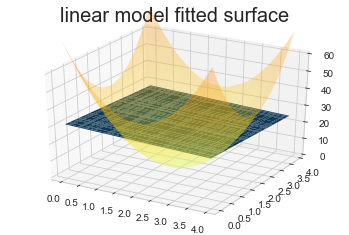
The basic linear regression model fits a linear function, \[z\sim w_1*x+w_2*y + b.\]
1
2
3
4
5
6
7
8
9
linearModel = tf.keras.models.Sequential([
    tf.keras.layers.Dense(1, input_dim = 2, kernel_initializer='normal', name = 'dense1')
])
linearModel.compile(optimizer = tf.keras.optimizers.Adam(learning_rate=0.01),
                   loss='mean_squared_error',
                   metrics=['mae'])

fithistory_linear = linearModel.fit(xmat, zvec, batch_size=128, verbose=0, epochs = 500)
fittedlinear = linearModel.predict(xmat).reshape(50, 50)
Obviously, the fitted \(z\) will just be a plane as in the following figure.
1
2
3
4
5
6
7
8
9
10
Model: "linearModel"
________________________________________
Layer (type)      Output Shape    Param
========================================
dense1 (Dense)    (None, 1)       3
========================================
Total params: 3
Trainable params: 3
Non-trainable params: 0
________________________________________
Model 2: 1 hidden layer with 20/40 units
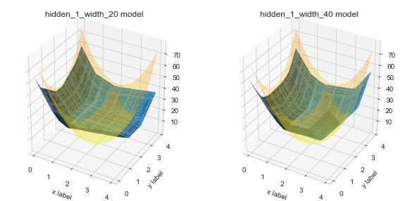
As in reference 1, we fit a shallow net with 1 hidden layer having 20/40 units. Even with dropout, the training process is not stable. After several trials, the loss function still can not reach the global minimum. As shown in the plot below, the blue fitted surface could have been closer to the truth. Also, the model has 81/161 parameters.
If we set the hidden layer has 20 units, since each Relu activation function folds the plane once, 20 Relu activations fold 20 planes which leads to a surface-wise constant function with 21 faces.
1
2
3
4
5
6
7
8
9
10
11
12
13
14
15
16
Model: "hidden1_width_20/40"
______________________________________________________
Layer (type)              Output Shape        Param #
======================================================
dense_2_to_20/40 (Dense) (None, 20/40)          60/120
______________________________________________________
re_lu (ReLU)             (None, 20/40)          0
______________________________________________________
dropout (Dropout)        (None, 20/40)          0
______________________________________________________
dense_20/40_to_1 (Dense) (None, 1)              21/41
======================================================
Total params: 81/161
Trainable params: 81/161
Non-trainable params: 0
______________________________________________________
Model 3: 2 hidden layers with 10 units
1
2
3
4
5
6
7
8
9
10
11
12
13
14
hidden_2_width_10 = tf.keras.models.Sequential([
    tf.keras.layers.Dense(10, input_dim = 2, kernel_initializer='normal', name = 'dense_2_to_10'),
    tf.keras.layers.ReLU(),
    tf.keras.layers.Dropout(0.5),
    tf.keras.layers.Dense(10,  kernel_initializer='normal', name = 'dense_10_to_10'),
    tf.keras.layers.ReLU(),
    tf.keras.layers.Dropout(0.5),
    tf.keras.layers.Dense(1, kernel_initializer='normal', name = 'dense_10_to_1')
])
hidden_2_width_10.compile(optimizer = tf.keras.optimizers.Adam(learning_rate=0.05),
                   loss='mean_squared_error',
                   metrics=['mae'])

fithistory_hidden_2_width_10 = hidden_2_width_10.fit(xmat, zvec, batch_size = 128, verbose=0, epochs = 500)
1
2
3
4
5
6
7
8
9
10
11
12
13
14
15
16
17
18
19
20
21
22
Model: "hidden2_width_10"
_________________________________________________________________
Layer (type)                 Output Shape              Param #
=================================================================
dense_2_to_10 (Dense)        (None, 10)                30
_________________________________________________________________
re_lu_60 (ReLU)              (None, 10)                0
_________________________________________________________________
dropout_37 (Dropout)         (None, 10)                0
_________________________________________________________________
dense_10_to_10 (Dense)       (None, 10)                110
_________________________________________________________________
re_lu_61 (ReLU)              (None, 10)                0
_________________________________________________________________
dropout_38 (Dropout)         (None, 10)                0
_________________________________________________________________
dense_10_to_1 (Dense)        (None, 1)                 11
=================================================================
Total params: 151
Trainable params: 151
Non-trainable params: 0
_________________________________________________________________
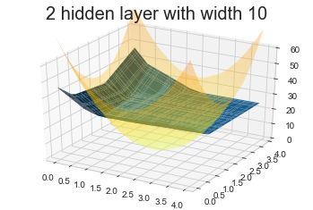
Though we have 151 parameters, but the fitted surface is far away from the truth, which is even worse than 1 hidden layer with 20 units (81 parameters).
Model 4: 3 hidden layers with 5 units
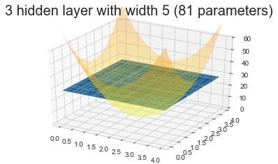
If we further make the Relu nets deeper to have 3 hidden layers, and each layer has 5 units, this will result in a net with 81 parameters. However, the final model is close to a purely linear model. Further investigation of the weight matrix reveals that all the fitted weights are much smaller than the weight in the 1 hidden layer models. Therefore, when the model is deeper, there are more plateaus in the objective function which makes the training very hard.
Model 5: 1 hidden 5 units + BatchNormalization
1
2
3
4
5
6
7
8
9
10
11
hidden_1_width_5_BN = tf.keras.models.Sequential([
    tf.keras.layers.Dense(5, input_dim = 2, kernel_initializer='normal', name = 'dense_2_to_5'),
    tf.keras.layers.BatchNormalization(),
    tf.keras.layers.ReLU(),
    tf.keras.layers.Dense(1, kernel_initializer='normal', name = 'dense_5_to_1')
])
hidden_1_width_5_BN.compile(optimizer = tf.keras.optimizers.Adam(learning_rate=0.1),
                   loss='mean_squared_error',
                   metrics=['mae'])

fithistory_hidden_1_width_5_BN= hidden_1_width_5_BN.fit(xmat, zvec, batch_size = 128, verbose=0, epochs = 500)
1
2
3
4
5
6
7
8
9
10
11
12
13
14
15
16
Model: "hidden_1_width_5_BN"
_________________________________________________________________
Layer (type)                 Output Shape              Param #
=================================================================
dense_2_to_5 (Dense)         (None, 5)                 15
_________________________________________________________________
batch_normalization (Batch)  (None, 5)                 20
_________________________________________________________________
re_lu (ReLU)                 (None, 5)                 0
_________________________________________________________________
dense_5_to_1 (Dense)         (None, 1)                 6
=================================================================
Total params: 41
Trainable params: 31
Non-trainable params: 10
_________________________________________________________________
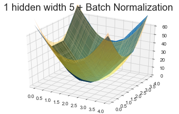
If we only have 1 hidden layer with only 5 units, adding the batch normalization not only enables convergence faster but also results in an excellent fit. Also, the total number of trainable parameters is 31, which is the smallest among all the above models.
Loss function in training stage
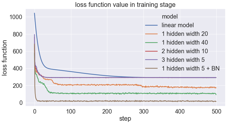
According to this simple post, models with batch normalization work the best even with the least number of parameters. Batch normalization not only accelerates the optimization procedure but also leads to an appropriate modeling structure. A more theoretical investigation of the batch normalization is necessary.
