Embedding algorithms 1 -- Multidimensional scaling

Manifold learning is a class of unsupervised estimators that seeks to describe datasets as low-dimensional manifolds embedded in high-dimensional spaces.

Some linear dimension reduction methods are: Independent component analysis (ICA), Principal component analysis (PCA) and Factor analysis.

Multidimensional scaling (MDS)

Given a matrix of pairwise ‘distances’ among a set of n objects or individuals”, MDS places each object into N-dimensional space such that the between-object distances are preserved as well as possible.

In the following, we will go through

• Classical MDS: when the distance matirx is Euclidean distance, cMDS is equivalent to PCA.
• Metric MDS: when the distance is not Euclidean, the stress loss function is based on scaled distance.
• Non-metric MDS: dissimilarities are known only by their rank order, we tend to preserve this order.
• Sparse distance matrix: when the distance matrix is sparse, we could first complete the distance matrix or only using the observed element when constructing the stress loss function.

Classical MDS

Suppose we observe

• \(\mathbf{Y} = [y_1, \ldots, y_n], y_i\in \mathbb{R}^d\)
• edm(\(\mathbf{Y}\)) the euclidean distance matrix created from columns in \(\mathbf{Y}\)
• distance/dissimilarity matrix \(\mathbf{D} = {d}_{ij}\)

MDS seeks to find \(x_1, \ldots, x_n\in \mathbb{R}^p\), called a configuration, so that \[d_{ij}\approx||x_i-x_j|| \text{ as close as possible.}\]

When the distance matrix \(D\) is edm(\(\mathbf{Y}\)), for large \(p\), there exists a configuration with exact/perfect distance match \(d_{ij}=\parallel x_i-x_j\parallel\). This is the case call classical MDS which is equivalent to PCA.

a) loss function:

cMDS try to solve \[\arg\min_{\mathbf{X}\in\mathbb{R}^{p\times n}}||\text{edm}(\mathbf{Y}) - \hat{D}||_F.\]

b) recover points from D:

When distance matrix is Euclidean distance, i.e. edm\((\mathbf{Y}) = \mathbf{D}\), it is invariant under rotation, reflection and translation (by adding a vector) of \(\mathbf{Y}\). In other words, from \(\mathbf{Y}\) to \(\mathbf{D}\), we only keep the reletive distance between \(y_i\) instead of actual coordinates. We will see that this is the reason of applying centering matrix on the both side of the Gram matrix \(\mathbf{G} = \mathbf{Y}^T\mathbf{Y}\), resulting in a row mean zero \(\mathbf{X}\).

\[\mathbf{D} = \text{edm}(\mathbf{Y}) = \mathbf{1}\text{diag}(\mathbf{Y}^T\mathbf{Y})^T - 2\mathbf{Y}^T\mathbf{Y}+ \text{diag}(\mathbf{Y^TY})\mathbf{1}^T\] Apply \(\mathbf{J} = \mathbf{I}-\frac{1}{n}\mathbf{11}^T\) on both sides, \[\mathbf{JDJ}^T = -2\mathbf{JY}^T\mathbf{YJ}^T = -2\mathbf{X}^T\mathbf{X}.\]

c) Algorithm-cMDS:

function cMDS(D, p)

\(\mathbf{J}\leftarrow \mathbf{I}-\frac{1}{n}\mathbf{11}^T,\text{ which is the centering matrix} \)
\(\mathbf{G}\leftarrow -\frac{1}{2}\mathbf{JDJ}^T\)
\(\mathbf{U}, (\lambda_i)_{i = 1}^n \leftarrow \text{EigenDecomp}(\mathbf{G})\)
\(\text{return [diag}(\sqrt{\lambda_1}, \ldots, \sqrt{\lambda_p}), \mathbf{0}]\mathbf{U}^T\)

d) cMDS in python:

1
2
3
4
5
6
7

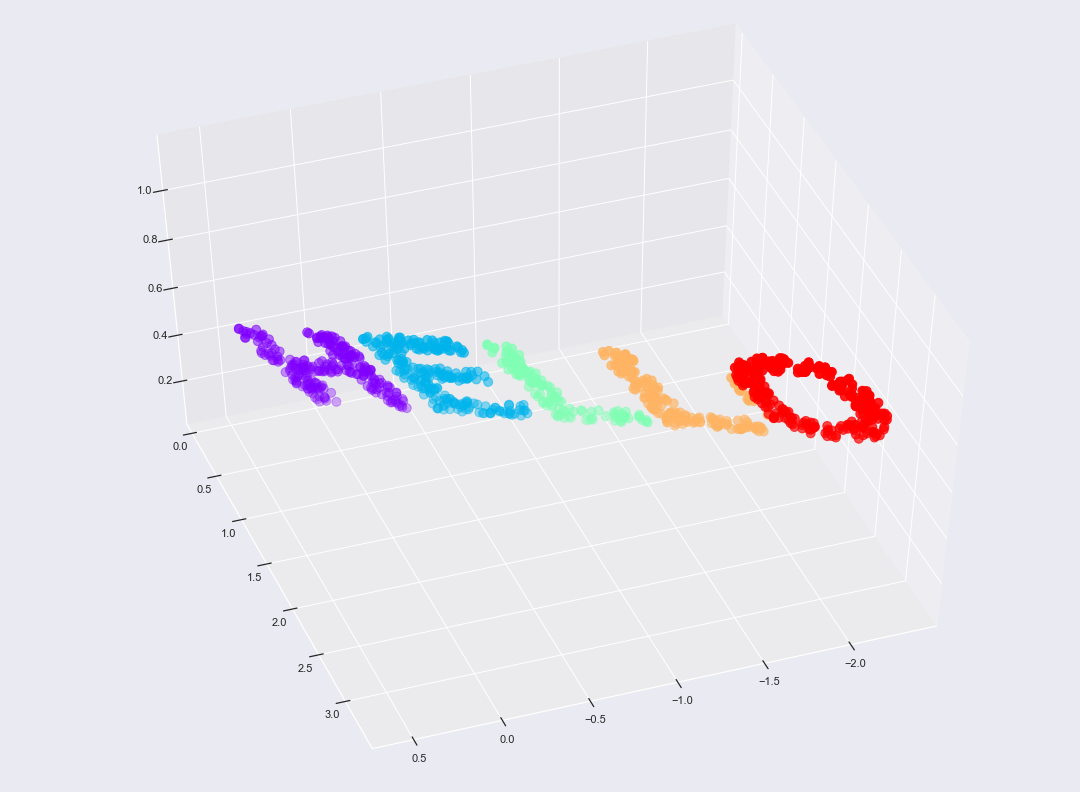
from mpl_toolkits import mplot3d
fig, ax = plt.subplots(figsize=(15, 11))
fig.subplots_adjust(left=0, right=1, bottom=0, top=1)
ax = plt.axes(projection='3d')
ax.scatter3D(X3[:, 0], X3[:, 1], X3[:, 2], **colorize, s = 80)
ax.view_init(azim=70, elev=50)
fig.savefig('hello3D.png')

1
2
3
4
5

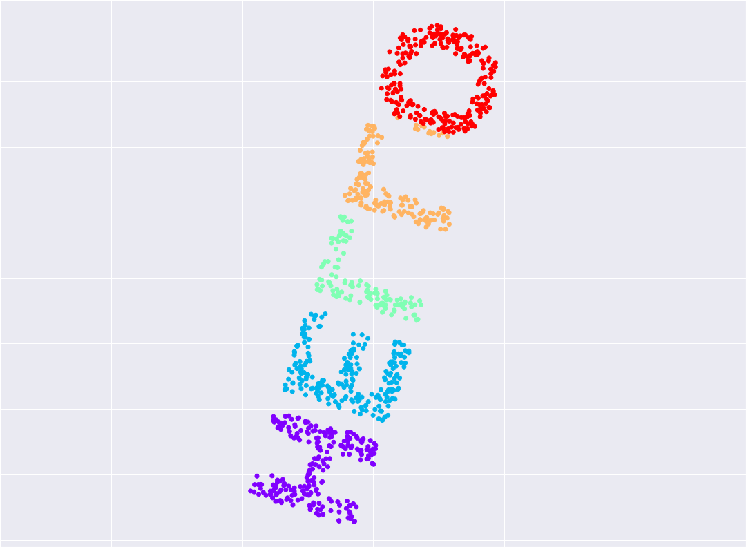
from sklearn.manifold import MDS            # 1. choose model class
model = MDS(n_components=2, random_state=1) # 2. instantiate model
out3 = model.fit_transform(X3)              # 3. fit the model
plt.scatter(out3[:, 0], out3[:, 1], **colorize)
plt.axis('equal');

Metric MDS

The general metric MDS relaxes the condition \(d_{ij} \approx \hat{d_{ij}}\) by allowing \(\hat{d_{ij}}\approx f(d_{ij})\), for some monotone function \(f\). Unlike cMDS, which has a explict solution, the general mMDS is an optimization process minimizing stress function, and is solved by iterative algorithms.

For instance, we could model \(f\) as a parametric monotonic function as \(f(d_{ij}) = \alpha + \beta d_{ij}\). Define the stress function as \[\text{stress} = \mathcal{L}(\hat{d_{ij}}) =\left(\frac{1}{\sum_{l<k} d_{lk}^2}\sum_{i<j} (\hat{d_{ij}} - f(d_{ij}))^2\right)^{1/2}\] and mMDS minimizes \(\mathcal{L}(\hat{d}_{ij})\) over all \(\mathbf{X}\) and \(\alpha, \beta\).

There are a pletora of modified stress loss functions. For instance, Sammon’s stress normalizes the squared-errors in pairwise distance by using the distance in the original space. As a result, Sammon mapping preserves the small \(d_{ij}\) better, giving them a greater degree of importance in the fitting procedure.

Non-metric MDS

In many applications, the dissimilarities are known only by their rank order.

• In this case, \(f\) is only implicitly defined.
• \(f(d_{ij}) = d_{ij}^\star\) are called dispartities, which only preserve the order of \(d_{ij}\), i.e., \[d_{ij} < d_{kl} \Leftrightarrow f(d_{ij})\leq f(d_{kl}) \Leftrightarrow d_{ij}^{\star}\leq d_{kl}^{\star}\]
• Kruskal’s non-metric MDS minimizes the stress-1 \[\text{stress-1}(\hat{d_{ij}}, d_{ij}^{\star}) = \left(\frac{1}{\sum_{l<k} d_{lk}^2} \sum_{i<j} (\hat{d_{ij}} - d_{ij}^\star)^2\right)^{1/2}.\]
• The original dissimilarites are only used in checking the order condition.

Sparse distance matrix

For advanced sparse distance matrix case, here is a useful reference, Euclidean Distance Matrices Essential Theory, Algorithms and Applications.