Embedding algorithms 2 -- Locally linear embedding

Introduction

In the last post, though the nonclassical/metric MDS is a nonlinear embedding algorithm, it is a global method (like PCA) since each point in the graph is related to all other \(n-1\) points in the reconstruction step. Locally linear embedding (LLE) is fundamentally different from those global methods. Essentially, when reconstructing the lower dimensional coordinates for one point, only the neighborhood information of this point is used. Put another way, the embedding is optimized to preserve the local configurations of the nearest neighbors.

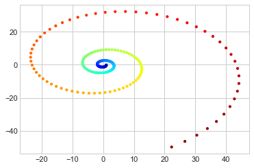
Below is a one-dimensional manifold lying in two-dimensional Euclidean space. The geometric structure can be embedded into a one-dimensional global coordinate– a straight line. However, we will see PCA as well as MDS ( remember they are equivalent in this case) will fail to learn the coordinate on the straight line.

1
2
3
4
5
6
7
8

import matplotlib.pyplot as plt
plt.style.use('seaborn-whitegrid')
import numpy as np

x_vec = np.exp(-0.2*(-np.arange(1, 201)/10))*np.cos(-np.arange(1, 201)/10)
y_vec = np.exp(-0.2*(-np.arange(1, 201)/10))*np.sin(-np.arange(1, 201)/10)
colorize = dict(c=np.arange(1, 201), cmap=plt.cm.get_cmap('jet', 201))
plt.scatter(x_vec, y_vec, s = 10,  **colorize)

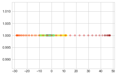
PCA can not capture the intrinsic nonlinear relationship in a swirl as we can see different color overlap with each other.

1
2
3
4
5
6

X = np.c_[x_vec, y_vec]
from sklearn.decomposition import PCA
pca = PCA(n_components=1)
pca.fit(X)
X_pca = pca.transform(X)
plt.scatter(X_pca, [1]*200, s = 30, alpha=0.3, **colorize)

Algorithm

The LLE algorithm has three steps:

Input:

• \(n\times D\) high-dimensional matrix \(\mathbf{X}\),
• an integer \(k\) used in the \(k\)-NN algorithm to define neighbors,
• the desired output dimension \(d\), where \(k\geq d+1\).

LLE algorithm:

1. For each \(\mathbf{x}_i\), find the \(k\) nearest neighbors.
2. Find the weight matirx \(\mathbf{W}\), which preserve the linear local information of each point.
3. Compute \(\mathbf{Y}\) which best fits the local pattern defined by the weight matrix \(\mathbf{W}\).

Output:

• \(n\times d\) low-dimensional matrix \(\mathbf{Y}\), which preserve the intrinsic coordinates of each point.

Step 1. Find nearest neighbors

The most commonly used algorithm to define a neighborhood is \(k\)-NN algorithm. An alternative method can be using a \(r\)-units ball. Essentially, \(k\) is a tuning parameter that governs trade-off between having enough points in each region (so as to deal with noise) and having small enough regions (to keep the linear approximation good.) In the summary paper written by Saul and Roweis, \(k\) has been set from 4 to 24. And they argued that in a range of \(k\) values, the performance of LLE should be stable and generally good.

Another crux is the relationship between \(k, d\) and \(D\). One definite relationship is \(d<D\) so we call LLE is a dimension reduction method.

• \(k \geq d+1\). The reason of this requirment is the \(k\) neighbors span a space of dimensionality at most \(k - 1\). Therefore, it is impossiable to use information less than \(d\) dimensions to construct \(d\)-dimensional points. Also, it was recommended that some margin between \(d\) and \(k\) is generally necessary to obtain a topology-preserving embedding.
• \(k\) can be greater or smaller than \(D\).
  1. \(k > D\) indicating the original data is low dimensional. Each point can be reconstructed perfectly from its neighbors, and the weights are no longer uniquely defined. Just think about we have \(D\) equations but \(k, k > D\), unknowns, so the solution is not unique. In this case, some regularization must be added to break the degeneracy.
  2. \(k < D\) is the usual case.

Step 2. Find Weights

The linearity of LLE comes form the weight finding step. For each point \(\mathbf{x}_i\), it is defined as a linear combination of its neighbors.

Then the weights are the optimizer of the cost function:

The second term in the cost function is the \(L_2\) regularizor, which encourages equal weights. The above optimization problem is subject to two constraints:

1. sparseness: if \(\mathbf{x}_{j}\) is out of the neighborhood of \(\mathbf{x}_i\), then \(w_{ij} = 0\).
2. invariance constraint: the local structure in the neighborhood should be invariance to translation, rotations and rescalings. Hence, \(\sum_j w_{ij} = 1\).

Indeed, the weigh finding step can be broken into \(n\) subproblems. Each is a least sqaure question subject to the sum to one condition, which could be easily solved by formulating a Lagrange multiplier question.

Step 3. Find coordinates

After finding the weight matrix \(\mathbf{W}\), it is used to represent the geometric information in \(\mathbf{X}\) so that \(\mathbf{X}\) does not appear in the final reconstruction step. The goal in this step is to find out \(n\times d, \mathbf{Y},\) matrix which minimizes

To break the degeneracy/make the optimization identifiable, the following assumptions are added:

1. \(\mathbf{Y}\) has column mean 0, i.e. \(\sum_i\mathbf{y}_{ij} = 0\).
2. \(\mathbf{Y}\) is an orthogonal matrix subject to a scaling factor, i.e. \(\frac{1}{n}\mathbf{Y}^T\mathbf{Y} = \mathbf{I}_d.\)

Since the geometric structure should be invariant under rotation, transformation (+/- constant), and homogeneously rescale the outputs, we can always make the covariance of \(\mathbf{Y}\) to be diagonal though the diagonal entris might be differ. The extra assumption is all the embedding coordinates should be of the same order.

The main difference between step 2 and step 3 is that step 3 is a global question so that the optimization question can not be seperated into small questions. It turns out the constrained optimization question is equivalent to find the smallest \(d+1\) eigenvector of a semipositive definite matrix. \[\Phi(\mathbf{Y}) = ||\mathbf{Y} - \mathbf{WY}||^2 = \text{trace}([(\mathbf{I} - \mathbf{W})\mathbf{Y}]^T[(\mathbf{I} - \mathbf{W})\mathbf{Y}]) = \text{trace}(\mathbf{Y}^T\mathbf{M}\mathbf{Y}).\]

First \(\mathbf{M}\) is a semipositive definite matrix and has 0 as an eigenvalue with \(\mathbf{1}\) as the corresponding eigenvector.

\[(\mathbf{I} - \mathbf{W})^T(\mathbf{I} - \mathbf{W})\mathbf{1} = (\mathbf{I} - \mathbf{W})^T(\mathbf{1} - \mathbf{1}) = 0 \text{ because of } \sum_jw_{ij} = 1.\]

Now form the Lagrange question \[L(\mathbf{Y}, \mu) = \text{trace}(\mathbf{Y}^T\mathbf{M}\mathbf{Y}) - \mu_1(\mathbf{Y}_1^T\mathbf{Y}_1 - n)-\ldots - \mu_d(\mathbf{Y}_d^T\mathbf{Y}_d - n).\] Take the first detivative with respect to \(\mathbf{Y}_i\), the ith column of \(\mathbf{Y}\), and set to be 0, \[\frac{\partial L(\mathbf{Y}, \mu)}{\mathbf{Y}_i} = 2 \mathbf{MY}_i - 2\mu_i\mathbf{Y}_i = 0.\] Finally, we get \(\mathbf{MY}_i = \mu_i \mathbf{Y}_i\). Thus, in order to minimize \(\Phi(\mathbf{Y})\), \(\mathbf{Y}_i\) should be the \(i+1\)th smallest eigenvector of \(\mathbf{M}\). Besides, the eigenvectors are orthogonal to each other and \(\mathbf{Y}_i\mathbf{1} = 0\) since \(\mathbf{1}\) is the eigenvector of eigenvalue 0, which means the columns of \(\mathbf{Y}\) have mean 0.

Implement in Python

1
2
3
4
5

from sklearn.manifold import LocallyLinearEmbedding
model = LocallyLinearEmbedding(n_neighbors=12, n_components=1, method='modified',
                               eigen_solver='dense')
lle_res = model.fit_transform(X)
plt.scatter(lle_res, [1]*200, s = 30, alpha=0.3, **colorize)

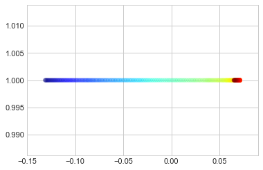
As we can see, the order of color in the above map is align with the color in swirl. So the linearity in a swirl is perfectly learned by LLE.

Reference:

1. CMU data mining lecture notes: Nonlinear Dimensionality Reduction I: Local Linear Embedding
2. Think Globally, Fit Locally: Unsupervised Learning of Low Dimensional Manifolds