
Multiple comparisons
In statistics, multiple comparisons/multiple hypothesis testing occurs when one considers a set of statistical inference questions simultaneously. To control the chance of making mistakes when the null hypotheses are true, one needs to control the family-wise error rate (FWER) or false discovery rate (FDR).
First, a confusion matrix can describe the possible outcomes when testing multiple null hypotheses. Suppose we have a number \(m \) of null hypotheses, denoted by \(H_1, H_2, \ldots, H_m\). The following table summaries the four types of outcomes.
| Null hypothesis is true | Alternative hypothesis is true | total | |
|---|---|---|---|
| test declares significant | V | S | R |
| test declares non-significant | U | T | m-R |
| total | \(m_0\) | \(m - m_0\) | m |
In the above table,
- V is the number of false positives, which is called the type I error;
- T is the number of false negatives, which is called the type II error.
In multiple comparisons,
- FWER = Pr(\(V\geq 1\)) = 1 - Pr(\(V=0\)), which is the probability of making at least one type I error.
- FDR = E[Q] = E\(\left[\frac{V}{V+S} \right]\) = E\(\left[\frac{V}{R} \right]\), where Q = 0 if R = 0. Thus, FDR is the expected proportion of false discoveries among all the discoveries. To exclude the case when R = 0, \[\text{FDR} = E[V/R|R=0]P(R = 0) + E[V/R|R>0]P( R > 0 ) = E[V/R|R>0]P(R>0).\]
Bonferroni correction
Bonferroni correction controls the FWER\(\leq \alpha\) without any assumptions about the dependence among the hypotheses questions. But the drawback is that it is very conservative if there are a large number of tests or the test statistics are positively correlated.
For hypothesis questions, the Bonferroni method rejects the null hypothesis if \(p_i\leq \frac{\alpha}{m}\). Then it follows,
\[\text{FWER} = P\left\{\cup_{i = 1}^{m_0} \left(p_i\leq \frac{\alpha}{m}\right)\right\} \leq\sum_{i=1}^{m_0}\left\{ P\left(p_i\leq\frac{\alpha}{m}\right)\right\} = m_0\frac{\alpha}{m}\leq\alpha.\]From the above derivation, we know that
- the first \(\leq\) reduces to = when the \(m_0\) questions are independent. If they are highly correlated, the probability of the union of the \(m_0\) events can be far less than the summation of the individual \(m_0\) probability, leading to a conservative conclusion.
- the second \(\leq\) reduces to = when all the null hypotheses are true in reality. We will see that the following Holm–Bonferroni method corrects \(\frac{\alpha}{m}\) to \(\frac{\alpha}{m_0}\).
Holm–Bonferroni method
Holm–Bonferroni method also intends to control the FWER but it is uniformly more powerful than the Bonferroni correction. By Bonferroni method, it control the FWER by adjusting the rejection criteria of each of the individual hypotheses.
1) Procedure:
- Let \(H_1, H_2, \ldots, H_m\) be a family of \(m\) null hypotheses and \(p_1, p_2, \ldots, p_m\) the corresponding p-values.
- Sort the p-values in increasing order, \(p_{(1)}, p_{(2)}, \ldots, p_{(m)}\) and the associated hypotheses are \(H_{(1)}, H_{(2)}, \ldots, H_{(m)}\).
- For a given significance level \(\alpha\), let \(k\) be the minimal index such that \(p_{(k)}>\frac{\alpha}{m+1-k}\).
- Reject the null hypothese \(H_{(1)}, \ldots, H_{(k-1)}\) and do not reject \( H_{(k)}, \ldots, H_{(m)}\).
This ensures the FWER\(\leq \alpha\).
2) Example:
Consider four null hypotheses \(H_1, \ldots, H_4\) with p-values \(p_1 = 0.01, p_2 = 0.04, p_3 = 0.03\) and \(p_4 = 0.005\) with test significance level \(\alpha = 0.05\).
| \(H_4\) | \(H_1\) | \(H_3\) | \(H_2\) |
|---|---|---|---|
| \(p_{(1)} = 0.005\) | \(p_{(2)} = 0.01\) | \(p_{(1)} = 0.03\) | \(p_{(1)} = 0.04\) |
| 0.05/4 = 0.0125 | 0.05/3 = 0.0167 | 0.05/2 = 0.25 | 0.05/1 = 0.05 |
| reject | reject | not reject | not reject |
3) Proof:
Let \(h\) be the first rejected true hypothesis. Then \(H_{(1)}, \ldots, H_{(h-1)}\) are all rejected false hypotheses and \(h-1\leq m -m_0\). Since \(h\) is rejected, we have \[p_{(h)}\leq \frac{\alpha}{m+1-h}\leq \frac{\alpha}{m_0}.\]
Thus, if we wrongly reject a true hypothesis, there has to be a true hypothesis with p-values at most \(\frac{\alpha}{m_0}\). Since we have total \(m_0\) true null hypotheses, the porbability of rejecting any of them is less than \(\alpha\). Thus, compared with the traditional Bonferroni method, it is obviously that the second \(\leq\) achieves =. Thus, it is less conservative then the simple bonferroni method.
Benjamini–Hochberg adjusted FDR p-values
1) Procedure:
- Let \(H_1, H_2, \ldots, H_m\) be a family of \(m\) null hypotheses and \(p_1, p_2, \ldots, p_m\) the corresponding p-values.
- Sort the p-values in increasing order, \(p_{(1)}, p_{(2)}, \ldots, p_{(m)}\) and the associated hypotheses are \(H_{(1)}, H_{(2)}, \ldots, H_{(m)}\).
- For a given \(\alpha\), find the largest \(k\) such that \(p_{(k)}\leq \frac{k}{m}\alpha\), or FRP adjusted p-value \(p_k^{*}\) = \(\min\left[p_{(k)}\frac{m}{k}, p_{k+1}^{*}\right]\), compared with \(\alpha\).
- Reject the null hypothese \(H_{(1)}, \ldots, H_{(k)}\).
2) Example:
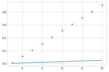
For instance, we have 10 p-values sorted in ascending order. We will notice that the FDR adjusted p-values are alway no less than the original p-values.
| p-values | 0.01 | 0.11 | 0.21 | 0.31 | 0.41 | 0.51 | 0.61 | 0.71 | 0.81 | 0.91 |
|---|---|---|---|---|---|---|---|---|---|---|
| rank | 1 | 2 | 3 | 4 | 5 | 6 | 7 | 8 | 9 | 10 |
| FDR adjusted p-values | 0.1 | 0.55 | 0.7 | 0.77 | 0.82 | 0.85 | 0.87 | 0.89 | 0.9 | 0.91 |
The smallest p-value is not less than 0.05. So we fail to reject any null hypothesis.
1
2
3
4
5
6
7
8
import matplotlib.pyplot as plt
plt.style.use('seaborn-whitegrid')
import numpy as np
alpha = 0.05
pvalues = [0.01, 0.11, 0.21, 0.31, 0.41, 0.51, 0.61, 0.71, 0.81, 0.91]
threshold = np.arange(1, 11) * 0.05/len(pvalues)
plt.plot(np.arange(1, 11), threshold)
plt.scatter(np.arange(1, 11), pvalues, marker='.', color='r')
Geometrically, all the p-values are above the line \(y = \frac{\alpha}{m}x\). We fail to reject any null hypothesis.
3) Proof:
The proof is given the original paper, reference 3. Here, I will only list the intuition of the FDR method.
When the null hypothesis is true, the realized/observed statistic, \(T*\) is a random variable from the sampling distribution, \(P_T\). Thus, the p-value \(P(T* > T), T\sim P_T\) is distributed as \(U(0, 1)\). This means about \(\alpha\times m_0\) cases will be false discoveries. At the same time, when the alternative hypthesis is true, the p-value is likely extremely small. The FDR adjusted/inflated p-values method hopefully makes the \(\alpha\times m_0\) p-values greater than \(\alpha\) and still keeps the extremely small p-values (from the S cases) less than \(\alpha\). The BH procedure controls the false discovery rate \(E[Q] \leq \frac{m_0}{m}\alpha\).
The BH procedure is valid when the \(m\) tests are independent or positive correlated. For general situations, there is a Euler-Mascheroni constant in \(\frac{k}{m\cdot c(m) }\alpha\) to further decrease the threshold. And this is the general Benjamini–Yekutieli procedure.