Sinkhorn Algorithm
The Wasserstein distance
The Wasserstein distance measures the discrepancy between two distributions. For simplicity, we consider discrete distributions on \([\delta_1, \delta_2, \ldots, \delta_n]\). Given a ground metric, for instance, the \(L_2 \) norm \(c(x, y) = \| x-y\|_2\), we are able to construct a distance matrix, \(\mathbf{C}_{i,j} = c(\delta^a_i, \delta^b_j)\). Then the p-Wasserstein distance between \(\mathbf{a}\) and \(\mathbf{b}\) is defined as
\[W_p(\mathbf{a}, \mathbf{b}) = \left(\min_{\mathbf{P}\in \mathbf{U}(\mathbf{a}, \mathbf{b})} \langle \mathbf{C}^{.p}, \mathbf{P}\rangle\right)^{1/p} = \left(\min_{\mathbf{P}\in \mathbf{U}(\mathbf{a}, \mathbf{b})} \sum_{i, j} \mathbf{C}^p_{i,j}\mathbf{P}_{i,j}\right)^{1/p},\]
where \(\mathbf{U}(\mathbf{a}, \mathbf{b}) = \{ \mathbf{P} \mid \sum_{i, j} \mathbf{P}_{i,j} = 1, \sum_{j}\mathbf{P}_{i, j} = \mathbf{a}, \sum_{i}\mathbf{P}_{i,j} = \mathbf{b} \}\) is the joint distribution over \([\delta^a_1, \delta^a_2, \ldots, \delta^a_n] \times [\delta^b_1, \delta^b_2, \ldots, \delta^b_n]\).
1
2
3
4
5
6
7
8
9
10
import random
import numpy as np
import cvxpy as cp
import holoviews as hv
from holoviews import opts
from bokeh.layouts import gridplot, row, column
from bokeh.plotting import figure, output_file, show
from bokeh.io import output_notebook, export_png
hv.extension('bokeh')
output_notebook()
1
2
3
4
5
6
7
8
9
10
11
12
13
14
15
16
17
18
### discretize a mixed normal distribution and gamma distribution ###
n_bins = 50
def mixedGaussian(mu1, mu2, sigma1, sigma2, n):
bernoulli = np.random.binomial(n = 1, p = 0.5, size = n)
gaussian1 = np.random.normal(mu1, sigma1, n)
gaussian2 = np.random.normal(mu2, sigma2, n)
return (gaussian1**bernoulli)*(gaussian2**(1-bernoulli))
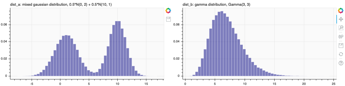
dist_a = mixedGaussian(mu1 = 1, mu2 = 10, sigma1 = 2, sigma2 = 1.5, n = 100000)
p_a, edges_a = np.histogram(dist_a, bins=n_bins)
pa = figure(title='dist_a: mixed gaussian distribution, 0.5*N(1, 2) + 0.5*N(10, 1.5)', background_fill_color="#fafafa", tools = "save", plot_height=300)
p_a = p_a/100000
pa.quad(top=p_a, bottom=0, left=edges_a[:-1], right=edges_a[1:], fill_color="navy", line_color="white", alpha=0.5)
dist_b = np.random.gamma(7, scale = 1, size = 100000)
p_b, edges_b = np.histogram(dist_b, bins=n_bins)
p_b = p_b/100000
pb = figure(title='dist_b: gamma distribution, Gamma(7, 1)', background_fill_color="#fafafa", y_range = pa.y_range, plot_height=300)
pb.quad(top=p_b, bottom=0, left=edges_b[:-1], right=edges_b[1:], fill_color="navy", line_color="white", alpha=0.5)
show(row(pa, pb)) #export_png(row(pa, pb), filename="sinkhorn428_p1.png")
This is a linear optimization problem since both the objective function and constriants are linear in \(\mathbf{P}\). Though the standard linear programming algorithms, like network simplex or interior point methods, work, the worst case complexity is \(O(n^3\log (n))\). Thus, with distributions in high-dimensional space or fine grid points (large n), the standard linear programming algorithms are not efficient.
1
2
3
4
5
6
7
8
9
10
11
12
13
14
15
16
17
18
19
20
###       linear programming to solve the Wasserstein distance       ###
edges_a = edges_a[:-1]
edges_b = edges_b[:-1]
# the distance matrix
C = (edges_a.reshape((n_bins,1)) - edges_b.reshape((1,n_bins)))**2
# Create two scalar optimization variables.
P0 = cp.Variable((n_bins, n_bins), nonneg=True)

# Create two constraints.
constraints = [cp.sum(P0, axis = 1) == p_a, cp.sum(P0, axis = 0) == p_b]

# Form objective.
obj = cp.Minimize(cp.trace(C.T@P0))

# Form and solve problem.
prob = cp.Problem(obj, constraints)
prob.solve()  # Returns the optimal value.
print("status:", prob.status)
print("optimal value", prob.value)
print("optimal var", P0.value)
Entropic regularization
Define the relative entropy between \(\mathbf{P}\) and \(\mathbf{a}\otimes\mathbf{b}\) as
\[\begin{align} KL(\mathbf{P} \mid \mathbf{a}\otimes\mathbf{b}) & = \sum_{i,j}\mathbf{P}_{i,j} \log \frac{ \mathbf{P}_{i,j} }{\mathbf{a}_i\times\mathbf{b}_j} \\
& = \sum_{i,j}\mathbf{P}_{i,j} \log \mathbf{P}_{i,j} - \sum_{i, j}\mathbf{P}_{i,j}\log \mathbf{a}_i\times\mathbf{b}_j \\
& = \sum_{i, j}\mathbf{P}_{i,j} \log \mathbf{P}_{i,j} - \sum_i\mathbf{a}_i\log \mathbf{a}_i-\sum_j\mathbf{b}_j\log\mathbf{b}_j , \end{align}\]
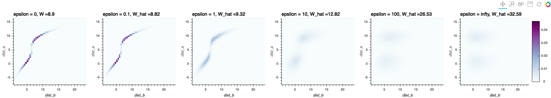
where \(\mathbf{a}\otimes\mathbf{b}\) denotes the joint distribution when the marginal distribution \(\mathbf{a} \text{ and } \mathbf{b}\) are independent. By the above derivation, regulization term \(KL(\mathbf{P} \mid \mathbf{a}\otimes\mathbf{b})\) is equivalent to \(- H(\mathbf{P}) = \sum_{i, j}\mathbf{P}_{i,j}\log \mathbf{P}_{i,j} - \mathbf{P}_{i,j}\) since the difference is a constant irrelevant to \(\mathbf{P}\). Then the entropic penalized Wasserstein distance is defined as \[ W_{\epsilon,p}^p = \min_{\mathbf{P}\in \mathbf{U}(\mathbf{a}, \mathbf{b})} \langle \mathbf{C}^{.p}, \mathbf{P}\rangle + \varepsilon KL(\mathbf{P}|\mathbf{a}\otimes\mathbf{b}) \] or \[ W_{\epsilon,p}^p = \min_{\mathbf{P}\in \mathbf{U}(\mathbf{a}, \mathbf{b})} \langle \mathbf{C}^{.p}, \mathbf{P}\rangle - \varepsilon H(\mathbf{P}). \] In the following, we list some properties of entropic penalized Wasserstein distance.
- Since \(KL(\mathbf{P}\mid\mathbf{a}\otimes\mathbf{b})\) is strongly convex, a unique minimizer exists in the above optimization problem. Note that the original Wasserstein distance in the Kantorovich formulation could have several minimizers.
- With the entropy regularization, the solution \(\mathbf{P}\) is less sparser in the sense that less number of \(\mathbf{P}_{i, j}\)’s are zero. Note that in the original Wasserstein distance, the solution \(\mathbf{P}\) of the linear programming lies on the boundary of \(\mathbf{U}(\mathbf{a}, \mathbf{b})\); that is, most of the entries of \(\mathbf{P}\) will be zeros.
- When \(\varepsilon\rightarrow\infty\), the solution \(\mathbf{P}\rightarrow \mathbf{a}\otimes\mathbf{b}\); when \(\varepsilon\rightarrow 0\), the solution \(\mathbf{P}\rightarrow \mathbf{P}^{OT}\).
Sinkhorn algorithm
In the following, we consider Wasserstein-2 distance, namely \(p = 2\). Then we relabel \(\mathbf{C}^{.2}\) as \(\mathbf{C}\). The Sinkhorn algorithm utilizes the dual formulation of the constrained convex optimization, which turns the unknown from \( \mathbf{P}\) (\(n^2\) unknowns) into the dual variables \(\mathbf{f}, \mathbf{g}\) (\(2n\) unknowns) of the linear constrants. Define the Lagrange function as \[ L(\mathbf{P}, \mathbf{f}, \mathbf{g}) = \langle \mathbf{C}, \mathbf{P} \rangle -\varepsilon H(\mathbf{P}) -\langle \mathbf{f}, \mathbf{P}\mathbb{1} - \mathbf{a}\rangle - \langle \mathbf{g}, \mathbf{P}^T\mathbb{1} - \mathbf{b}\rangle. \] The first order condition is \[ \frac{\partial L(\mathbf{P}, \mathbf{f}, \mathbf{g})}{\partial \mathbf{P}_{i,j}} = \mathbf{C}_{i,j}+\varepsilon \log \mathbf{P}_{i,j}-\mathbf{f}_i - \mathbf{g}_j = 0, \] which leads to the solution \[ \mathbf{P} = \text{diag}(e^{\mathbf{f}/\varepsilon}) * e^{\frac{-\mathbf{C}}{\varepsilon}} * \text{diag}(e^{\mathbf{g}/\varepsilon}). \] Therefore, the solution must be in the form of \[\text{diag}(\mathbf{u})* \mathbf{K}* \text{diag} (\mathbf{v}), \mathbf{K} = e^{\frac{-\mathbf{C}}{\varepsilon}}.\] The marginal constraints require \[ \text{diag}(\mathbf{u})* \mathbf{K}* \text{diag} (\mathbf{v}) \mathbb{1} = \mathbf{a} \text{ and } \text{diag}(\mathbf{v})* \mathbf{K}^T * \text{diag} (\mathbf{u}) \mathbb{1} = \mathbf{b}. \]
Input: \(\mathbf{C}, \mathbf{a}, \mathbf{b}, \varepsilon\)
- Initialization: \(\mathbf{u} = \mathbf{v} = \mathbb{1}, \mathbf{K} = e^{\frac{-\mathbf{C}}{\varepsilon}}\).
- Main loop:
While \(\|\mathbf{P}\|\) changes do:
\(\mathbf{u}^{(i+1)} = \frac{\mathbf{a}}{\mathbf{K}*\mathbf{v}^{(i)}}\text{ and }\mathbf{v}^{(i+1)} = \frac{\mathbf{b}}{\mathbf{K}^T*\mathbf{u}^{(i+1)}}\)
Return: \(\mathbf{P} = \mathbf{u}*\mathbf{K}*\mathbf{v}\), \(\widehat{W}^p_{p} = \text{trace}(\mathbf{C}^T\mathbf{P})\)
1
2
3
4
5
6
7
8
9
10
11
12
13
14
15
16
17
18
19
20
element_max = np.vectorize(max)
def sinkhorn(C, a, b, epsilon, precision):
    a = a.reshape((C.shape[0], 1))
    b = b.reshape((C.shape[1], 1))
    K = np.exp(-C/epsilon)

    # initialization
    u = np.ones((C.shape[0], 1))
    v = np.ones((C.shape[1], 1))
    P = np.diag(u.flatten()) @ K @ np.diag(v.flatten())
    p_norm = np.trace(P.T @ P)

    while True:
        u = a/element_max((K @ v), 1e-300) # avoid divided by zero
        v = b/element_max((K.T @ u), 1e-300)
        P = np.diag(u.flatten()) @ K @ np.diag(v.flatten())
        if abs((np.trace(P.T @ P) - p_norm)/p_norm) < precision:
            break
        p_norm = np.trace(P.T @ P)
    return P, np.trace(C.T @ P)
1
2
###       apply sinkhorn algorithm to epsilon = 0.1, 1, 10, 100       ###
P1, W_1 = sinkhorn(C, p_a, p_b, epsilon = 1, precision = 1e-30)
1
2
3
4
5
6
7
8
9
10
###       visualize the join distribution with different epsilon       ###
bounds=(edges_b.min(), edges_a.min(), edges_b.max(), edges_a.max())   # Coordinate system: (left, bottom, right, top)
img_0 = hv.Image(np.flip(P0.value, axis=0), bounds=bounds).relabel("epsilon = 0" + ', W =' + str(round(prob.value, 2))).opts(colorbar=False, cmap = 'BuPu', color_levels = int(1e4), width=300, xlabel='dist_b', ylabel='dist_a').redim.range(z = (0, np.max(P0.value)))
img_01 = hv.Image(np.flip(P01, axis=0), bounds=bounds).relabel((', ').join(["epsilon = 0.1",  'W_hat =' + str(round(W_01, 2))])).opts(colorbar=False, cmap = 'BuPu', color_levels = int(1e4), width=300, xlabel='dist_b', ylabel='dist_a').redim.range(z = (0, np.max(P0.value)))

P_independent = p_a.reshape((n_bins, 1))*p_b.reshape((1, n_bins))
img_infty = hv.Image(np.flip(P_independent, axis = 0), bounds=bounds).relabel((', ').join(["epsilon = infty",  'W_hat =' + str(round(np.trace(C.T @ P_independent), 2))])).opts(colorbar=True, cmap = 'BuPu', color_levels = int(1e4), width=350, xlabel='dist_b', ylabel='dist_a').redim.range(z = (0, np.max(P0.value)))

layout = hv.Layout([img_0, img_01, img_1, img_10, img_100, img_infty]).cols(6)
hv.save(layout, filename="sinkhorn428_p2.png")